Some animations of line integrals

Evaluating a line integral $\int_C F \cdot dr$ requires two pieces of data:

A curve $C$ parametrized by some function $r(t)=(x(t),y(t))$ with $t$ ranging from (say) $0$ to $1$ .
A vector field $F(x,y)=(P(x,y),Q(x,y))$ .

Then the line integral is

$\int_C F\dot dr=\int_0^1 \left[P(r(t)) x'(t)+Q(r(t))y'(t)\right] dt,$

which is just the integral of a scalar valued function of one variable. From earlier courses in calculus, we visualize the latter as ‘area under the curve,’ or perhaps the ‘average value.’

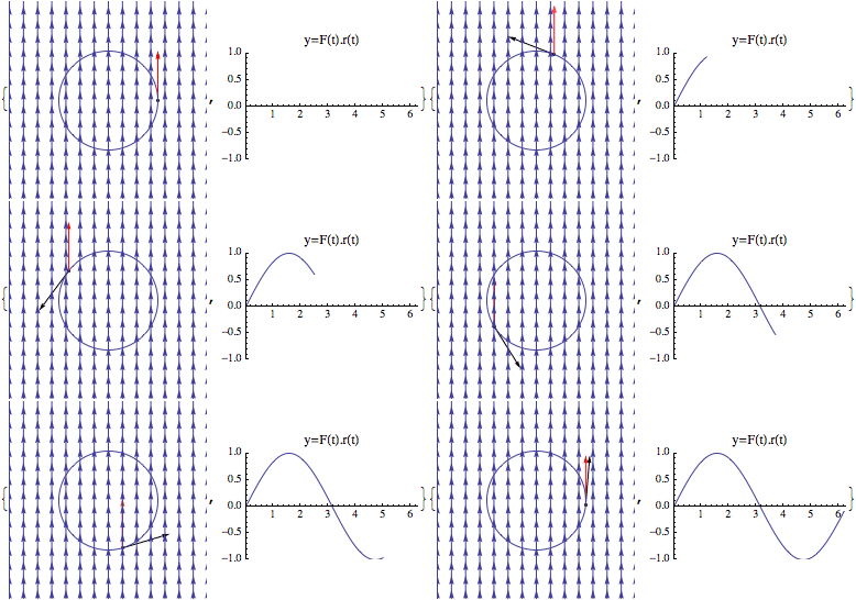
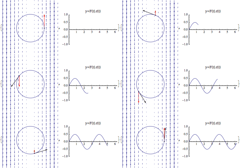
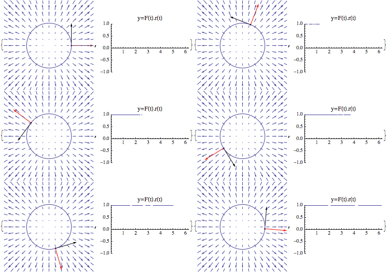
The following animations show how the scalar valued function on the right hand side of the equality above comes from the 2-dim’l scenario. The values graphed on the left are the values of the dot product between the red vector, $F(r(t))$ and the tangent vector to the curve $r(t)$ at time $t$ .

Here the integral is over the unit circle, and the vector field is the constant function .
With the same curve, the vector field is
With respect to the same curve, the vector field is

Share this: